使用Librosa库对音乐速度、节拍进行估计的基本方法

参考:https://tempobeatdownbeat.github.io/tutorial/ch2_basics/baseline.html

基本设置

1
2
3
4
import librosa
import matplotlib.pyplot as plt
import librosa.display
import numpy as np
1
mount = False
1
2
3
4
from google.colab import drive
drive.mount('/content/drive')
# drive._mount('/content/drive') # failed on Jan 21st, 2022
mount = True
1
2
3
4
5
6
7
8
9
10
11
12
13
14
if mount == True:
filename = "drive/MyDrive/data/tempo_tutorial/audio/book_assets_ch2_basics_audio_easy_example"
else:
filename = "book_assets_ch2_basics_audio_easy_example"
sr = 44100
fps = 100
hop_length = int(librosa.time_to_samples(1./fps,sr=sr)) # 441
# this Calculation is new to me
n_fft = 2048
# length of fft window
fmin = 27.5
fmax = 17000.
n_mels = 80
# number of Mel bands to generate
1
y, sr = librosa.load(filename+".flac", sr=sr)

时频特征(Mel-Spectrogram)

1
2
3
4
5
6
7
8
9
10
11
# Mel-spectrogram
mel_spec = librosa.feature.melspectrogram(y, sr=sr, n_fft=n_fft,
hop_length=hop_length,
fmin=fmin, fmax=fmax,
n_mels=n_mels)
# melspectrogram's defult parameters
# fmax = sr / 2
# win_length = n_fft
# power = 2 # exponent for the magnitude melspectrogram. e.g., 1 for energy, 2 for power, etc.

# If a time-series input y, sr is provided, then its magnitude spectrogram S is first computed, and then mapped onto the mel scale by mel_f.dot(S**power).
1
2
3
4
5
6
7
8
9
10
11
12
13
fig, ax = plt.subplots(nrows=2, sharex=True, figsize=(14,6))
librosa.display.waveplot(y, sr=sr, alpha=0.6, ax=ax[0])
# alpha controls the color transparency
ax[0].set_title('Audio waveform', fontsize=15)
ax[0].label_outer()
# only show "outer" labels and tick labels

librosa.display.specshow(librosa.power_to_db(mel_spec, ref=np.max), # convert a power spectrogram (amplitude(?) squared) to decibel (dB) units
y_axis='mel', x_axis='time', sr=sr,
hop_length=hop_length, fmin=fmin, fmax=fmax,
ax=ax[1])
ax[1].set_title('Mel Spectrogram', fontsize=15)
ax[1].label_outer()

png

中层特征(Spectral Flux)

1
2
3
4
5
6
7
8
9
10
11
12
13
14
15
16
17
18
19
20
21
22
23
# Mid-level Representation (Spectral Flux)

# Onset strength at time t is determined by:
# mean_f max(0, S[f, t] - ref[f, t - lag])
# where ref is S after local max filtering along the frequency axis.

S = mel_spec # pre-computed (log-power) spectrogram
lag = 2 # time lag for computing differences
max_size = 3 # size (in frequency bins) of the local max filter, set to 1 to disable filtering
spectral_flux = librosa.onset.onset_strength(S=librosa.power_to_db(S, ref=np.max),
sr=sr, hop_length=hop_length,
lag=lag, max_size=max_size)
# Compute a spectral flux onset strength envelope

times = librosa.frames_to_time(np.arange(len(spectral_flux)),
sr=sr, hop_length=hop_length)
# or librosa.times_like(spectral_flux, sr=sr, hop_length=hop_length)

plt.figure(figsize=(14, 3))
plt.plot(times, spectral_flux, label="Spectral flux")
plt.title("Spectral flux")
plt.legend() # show legend
plt.show()

png

速度估计(Autocorrelation)

1
2
3
4
5
6
7
8
9
10
11
12
13
14
15
16
17
18
19
20
21
22
23
24
25
26
27
28
29
30
31
32
33
34
35
36
37
38
39
40
41
42
43
44
45
46
47
48
49
50
51
52
53
54
55
56
57
58
59
60
61
62
63
64
65
66
67
68
69
# Periodicity Detection and Tempogram

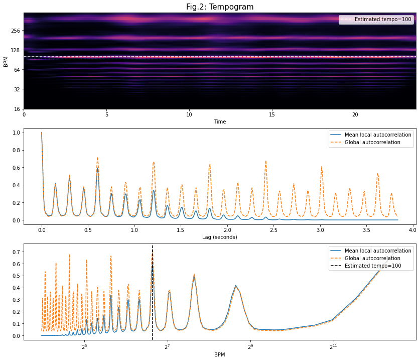
fig, ax = plt.subplots(nrows=3, figsize=(14, 12))

tempogram = librosa.feature.tempogram(onset_envelope=spectral_flux,
sr=sr, hop_length=hop_length)
# Compute the tempogram: local autocorrelation of the onset strength envelope
# default win_length = 384: length of the onset autocorrelation window
# return_shape = (win_length, n)
# time lag changes from 0 to win_length (?) \
# when time_lag == win_length \
# there is no overlap between origin window and shifted window, thus autocorrelation should be 0 \
# but for global_ac (window is much larger) there are still a lot of overlops

librosa.display.specshow(tempogram, sr=sr, hop_length=hop_length,
x_axis='time', y_axis='tempo', cmap='magma',
ax=ax[0])
# y_axis='tempo' visualizes the outputs of feature.tempogram
# cmap: color map
# win_length => BPM (?)

tempo = librosa.beat.tempo(onset_envelope=spectral_flux, sr=sr,
hop_length=hop_length)[0]
# default aggregation function: mean
# shape = (1,) or (n,) if no aggregate
ax[0].axhline(tempo, color='w', linestyle='--', alpha=1,
label='Estimated tempo={:g}'.format(tempo))
# this line shows the estimated global tempo
ax[0].legend(loc='upper right')
ax[0].set_title('Fig.2: Tempogram',fontsize=15)

ac_global = librosa.autocorrelate(spectral_flux, max_size=tempogram.shape[0])
# Compute global onset autocorrelation
# max_size: maximum correlation lag
ac_global = librosa.util.normalize(ac_global)

x_scale = np.linspace(start=0, stop=tempogram.shape[0] * float(hop_length) / sr,
num=tempogram.shape[0])
# return evenly spaced numbers over a specified interval
ax[1].plot(x_scale, np.mean(tempogram, axis=1), label='Mean local autocorrelation')
ax[1].plot(x_scale, ac_global, '--', label='Global autocorrelation')
ax[1].legend(loc='upper right')
ax[1].set(xlabel='Lag (seconds)')

# ax[2]: map the lag scale into tempo, which is a prior distribution
freqs = librosa.tempo_frequencies(n_bins = tempogram.shape[0],
hop_length=hop_length, sr=sr)
# Compute the frequencies (in beats per minute) corresponding to an onset auto-correlation or tempogram matrix
# n_bins: the number of lag bins
# freqs[0] = +np.inf corresponds to 0-lag
# freqs[1] = 6000, [2] = 3000, [3] = 1500 ...
# freqs here means x_scale

ax[2].semilogx(freqs[1:], np.mean(tempogram[1:], axis=1),
label='Mean local autocorrelation', basex=2)
ax[2].semilogx(freqs[1:], ac_global[1:], linestyle='--',
label='Global autocorrelation', basex=2)
ax[2].axvline(tempo, color='black', linestyle='--',
label='Estimated tempo={:g}'.format(tempo))

ax[2].legend(loc='upper right')
ax[2].set(xlabel='BPM')
# blue line taper off at higher periodicity (lower tempi) \
# due to the lack of overlap between the shifted versions of the windowed spectral flux

plt.show()

# Notice that in a variable tempo context, \
# it’s not super meaningful to reduce the tempo information down to a single value.

png

节拍跟踪(Dynamic Programming)

1
2
3
4
5
6
7
8
9
10
11
12
13
14
15
16
17
18
19
20
21
22
23
24
25
26
27
28
29
30
31
32
33
34
35
36
37
38
39
40
41
42
43
44
45
46
47
48
49
50
51
52
53
54
55
56
57
58
59
60
61
62
63
64
65
66
67
68
69
70
71
72
73
74
75
76
77
# Use DP to recover beats sequence (i.e., temporal locations)
# Ref: https://www.audiolabs-erlangen.de/resources/MIR/FMP/C6/C6S3_BeatTracking.html
'''
Pseudocode:
for i = 1 to N
int tmp = 0;
for j = 1 to i-1
tmp = max(tmp, dp[j] + lamda * penalty(i-j));
dp[i] = delta[i] + tmp

'''
def beat_track_dp(oenv, tempo, fps, sr, hop_length, tightness=100, alpha=0.5, ref_beats=None):

period = (fps * 60./tempo) # beat period (given in samples)
localscore = librosa.beat.__beat_local_score(oenv, period)
"""Construct the local score for an onset envlope and given period"""
# localscore is a smoothed version of AGC'd(?) onset envelope

backlink = np.zeros_like(localscore, dtype=int) # save answers in DP process
cumulative_score = np.zeros_like(localscore)

# Search range for previous beat
window = np.arange(-2 * period, -np.round(period / 2) + 1, dtype=int)

txwt = -tightness * (np.log(-window / period) ** 2)
# penalty function
# notice window is an array, so txwt saves not only one penalty value
# tightness means tightness of beat distribution around tempo
# higher tightness value favours constant tempi

# Are we on the first beat?
first_beat = True
for i, score_i in enumerate(localscore):

# Are we reaching back before time 0?
z_pad = np.maximum(0, min(-window[0], len(window)))

# Search over all possible predecessors
candidates = txwt.copy()
candidates[z_pad:] = candidates[z_pad:] + cumulative_score[window[z_pad:]]

# Find the best preceding beat
beat_location = np.argmax(candidates)

# Add the local score
cumulative_score[i] = (1-alpha)*score_i + alpha*candidates[beat_location]

# Special case the first onset. Stop if the localscore is small
if first_beat and score_i < 0.01 * localscore.max():
backlink[i] = -1
else:
backlink[i] = window[beat_location]
first_beat = False

# Update the time range
window = window + 1

beats = [librosa.beat.__last_beat(cumulative_score)]
"""Get the last beat from the cumulative score array"""
# get the last (final) beat

# Reconstruct the beat path from backlinks
while backlink[beats[-1]] >= 0:
beats.append(backlink[beats[-1]])

# Put the beats in ascending order
# Convert into an array of frame numbers
beats = np.array(beats[::-1], dtype=int)

# Discard spurious trailing beats
beats = librosa.beat.__trim_beats(oenv, beats, trim=True)
"""Final post-processing: throw out spurious leading/trailing beats"""

# Convert beat times seconds
beats = librosa.frames_to_time(beats, hop_length=hop_length, sr=sr)

return beats, cumulative_score
1
2
3
4
5
6
7
8
9
10
11
12
13
14
15
16
17
18
19
20
21
22
23
24
alpha = 0.5
tightness=100

est_beats, cumulative_score = beat_track_dp(oenv=spectral_flux, tempo=tempo, fps=fps, sr=sr, hop_length=hop_length, tightness=tightness, alpha=alpha)
fig, ax = plt.subplots(nrows=2, figsize=(14, 6))
times = librosa.times_like(spectral_flux, sr=sr, hop_length=hop_length)
ax[0].plot(times, spectral_flux, label='Spectral flux')
ax[0].set_title('Spectral flux',fontsize=15)
ax[0].label_outer()

ax[0].set(xlim=[0, len(spectral_flux)/fps])
ax[0].vlines(est_beats, 0, 1.1*spectral_flux.max(), label='Estimated beats',
color='green', linestyle=':', linewidth=2)
ax[0].legend(loc='upper right')

ax[1].plot(times, cumulative_score, color='orange', label='Cumultative score')
ax[1].set_title('Cumulative score (alpha:'+str(alpha)+')',fontsize=15)
ax[1].label_outer()
ax[1].set(xlim=[0, len(spectral_flux)/fps])
ax[1].vlines(est_beats, 0, 1.1*cumulative_score.max(), label='Estimated beats',
color='green', linestyle=':', linewidth=2)
ax[1].legend(loc='upper right')
ax[1].set(xlabel = 'Time')
plt.show()

png